About
Unstructured data, such as text, images, and audio, varies in format and carries rich underlying semantics, making it challenging to analyze. To manage this complexity, embeddings are used to convert unstructured data into numerical vectors that capture its essential characteristics. These vectors are then stored in a vector database, enabling fast and scalable searches and analytics.
- Milvus Lite is a Python library that can be easily integrated into your applications. As a lightweight version of Milvus, it’s ideal for quick prototyping in Jupyter Notebooks or running on edge devices with limited resources. Learn more.
- Milvus Standalone is a single-machine server deployment, with all components bundled into a single Docker image for convenient deployment. Learn more.
- Milvus Distributed can be deployed on Kubernetes clusters, featuring a cloud-native architecture designed for billion-scale or even larger scenarios. This architecture ensures redundancy in critical components. Learn more.
High performance
Hardware-aware Optimization
Advanced Search Algorithms
C++ Search Engine
Column-Oriented
The primary advantages come from the data access patterns. When performing queries, a column-oriented database reads only the specific fields involved in the query, rather than entire rows, which greatly reduces the amount of data accessed. Additionally, operations on column-based data can be easily vectorized, allowing for operations to be applied in the entire columns at once, further enhancing performance.
Architecture
Milvus itself is fully stateless so it can be easily scaled with the help of Kubernetes or public clouds.
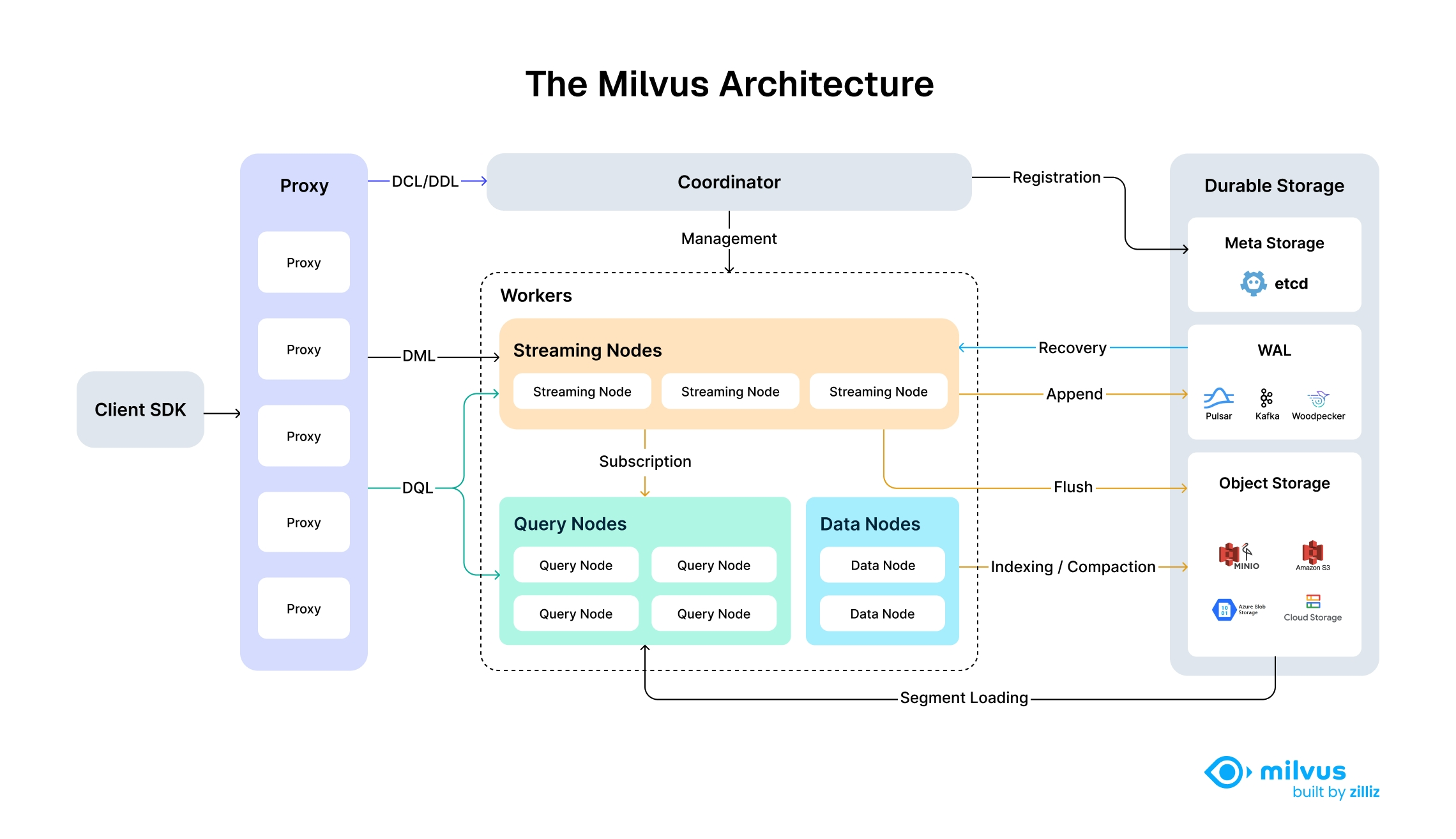 Milvus follows the principle of data plane and control plane disaggregation, comprising four main layers that are mutually independent in terms of scalability and disaster recovery.
Access Layer
Composed of a group of stateless proxies, the access layer is the front layer of the system and endpoint to users. It validates client requests and reduces the returned results.
Coordinator
The Coordinator serves as the brain of Milvus. At any moment, exactly one Coordinator is active across the entire cluster, responsible for maintaining the cluster topology, scheduling all task types, and promising cluster-level consistency.
Worker Nodes
Worker nodes are stateless thanks to separation of storage and computation, and can facilitate system scale-out and disaster recovery when deployed on Kubernetes.
Streaming Node
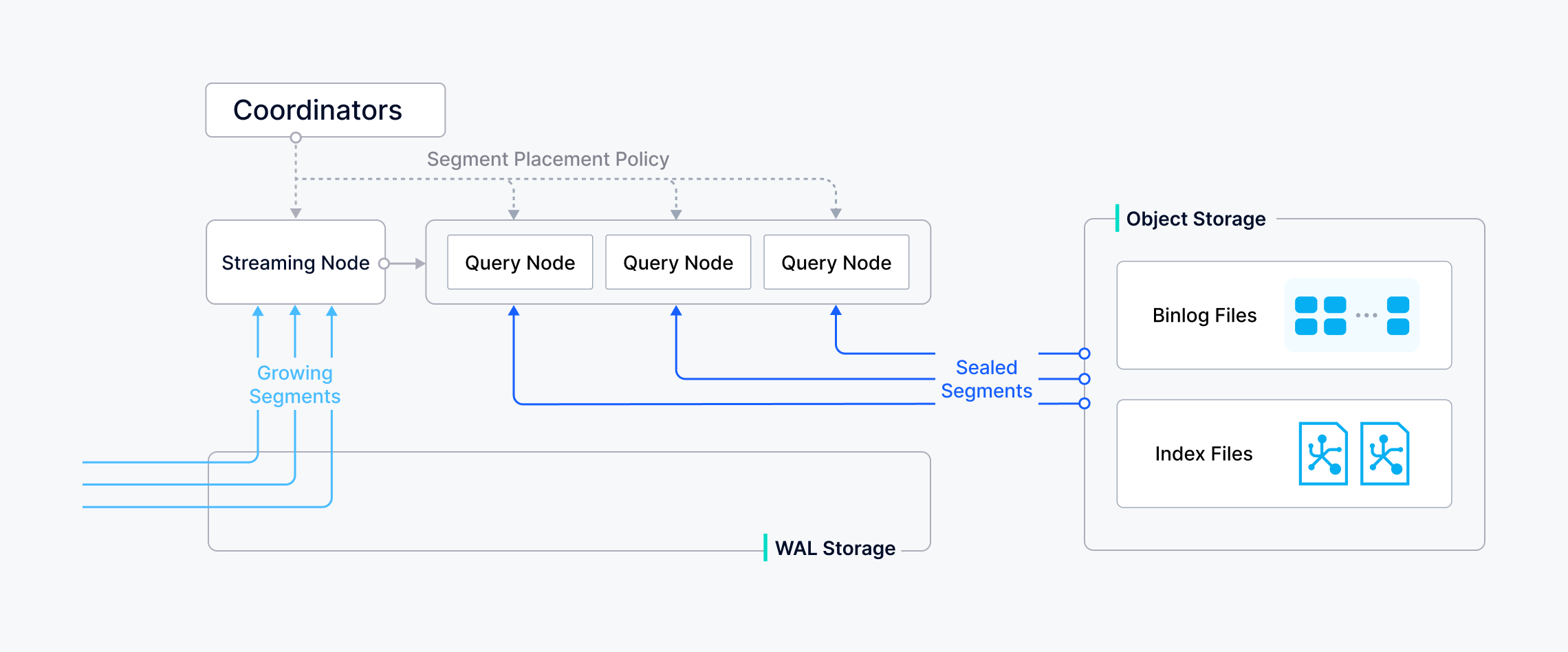
Streaming Node serves as the shard-level “mini-brain”, providing shard-level consistency guarantees and fault recovery based on underlying WAL Storage. Meanwhile, Streaming Node is also responsible for growing data querying and generating query plans. Additionally, it also handles the conversion of growing data into sealed (historical) data.
Data Node
Data node is responsible for offline processing of historical data, such as compaction and index building.
Query Node
Query node loads the historical data from object storage, and provides the historical data querying.
Storage
Storage is the bone of the system, responsible for data persistence. It comprises meta storage, log broker, and object storage.
Meta Storage (etcd)
Meta storage stores snapshots of metadata such as collection schema, and message consumption checkpoints.
Object Storage
Object storage stores snapshot files of logs, index files for scalar and vector data, and intermediate query results. Milvus uses MinIO as object storage and can be readily deployed on AWS S3 and Azure Blob, two of the world’s most popular, cost-effective storage services.
WAL Storage
| API Category | Operations | Example APIs | Architecture Flow |
|---|---|---|---|
| DDL/DCL | Schema & Access Control | createCollection, dropCollection, hasCollection, createPartition | Access Layer → Coordinator |
| DML | Data Manipulation | insert, delete, upsert | Access Layer → Streaming Worker Node |
| DQL | Data Query | search, query | Access Layer → Batch Worker Node (Query Nodes) |
Data Flow
Search:
- Client sends a search request via SDK/RESTful API
- Load Balancer routes request to available Proxy in Access Layer
- Proxy uses routing cache to determine target nodes; contacts Coordinator only if cache is unavailable
- Proxy forwards request to appropriate Streaming Nodes, which then coordinate with Query Nodes for sealed data search while executing growing data search locally
- Query Nodes load sealed segments from Object Storage as needed and perform segment-level search
- Search results undergo multi-level reduction: Query Nodes reduce results across multiple segments, Streaming Nodes reduce results from Query Nodes, and Proxy reduces results from all Streaming Nodes before returning to client
Insert:
- Client sends an insert request with vector data
- Access Layer validates and forwards request to Streaming Node
- Streaming Node logs operation to WAL Storage for durability
- Data is processed in real-time and made available for queries
- When segments reach capacity, Streaming Node triggers conversion to sealed segments
- Data Node handles compaction and builds indexes on top of the sealed segments, storing results in Object Storage
- Query Nodes load the newly built indexes and replace the corresponding growing data
Streaming Service
The Streaming Service is a concept for Milvus internal streaming system module, built around the Write-Ahead Log (WAL) to support various streaming-related function.
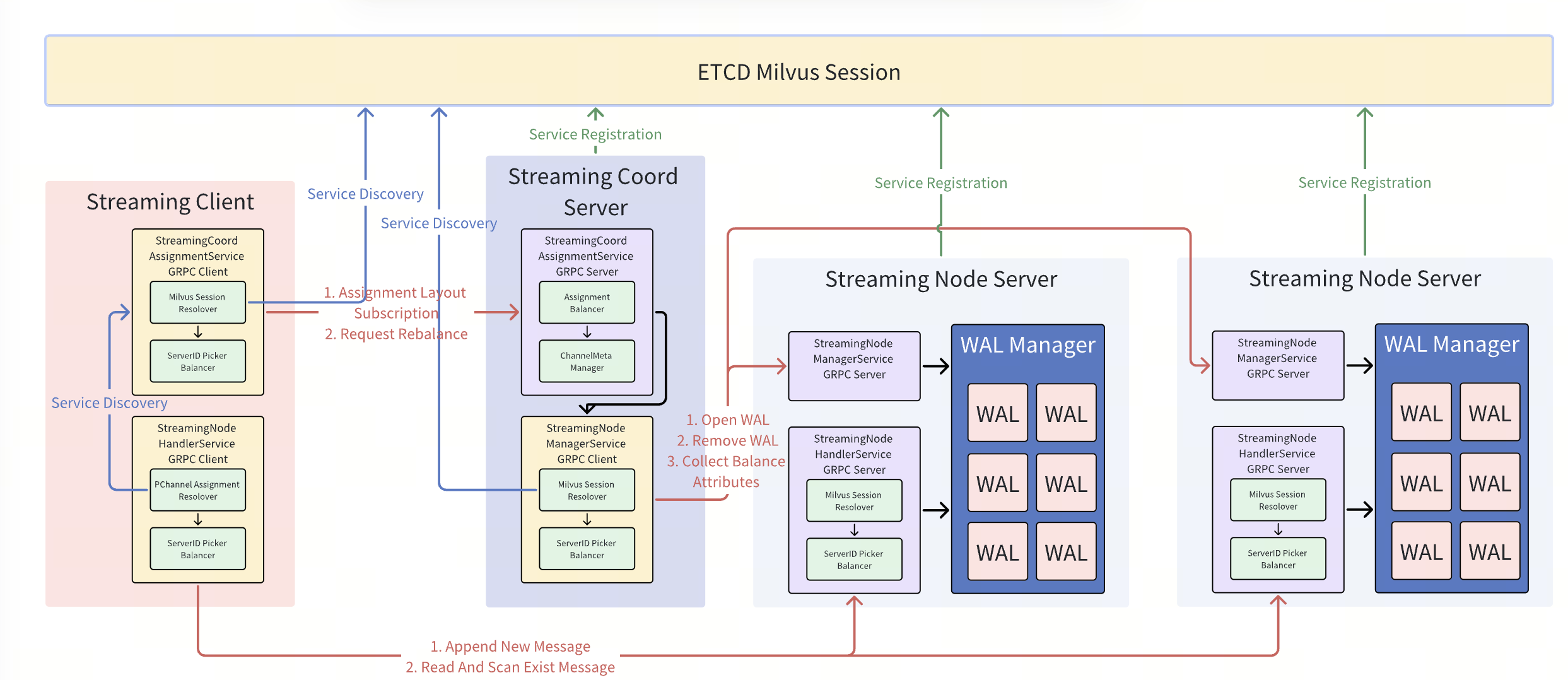
- Streaming Coordinator: A logical component in the coordinator node. It uses Etcd for service discovery to locate available streaming nodes and is responsible for binding WAL to the corresponding streaming nodes. It also registers service to expose the WAL distribution topology, allowing streaming clients to know the appropriate streaming node for a given WAL.
- Streaming Node Cluster: A cluster of streaming worker nodes responsible for all streaming-processing tasks, such as wal appending, state recovering, growing data querying.
- Streaming Client: An internally developed Milvus client that encapsulates basic functionalities such as service discovery and readiness checks. It is used to initiate operations such as message writing and subscription.
Message
The Streaming Service is a log-driven streaming system, so all write operations in Milvus (such as DML and DDL) are abstracted as Messages.
- Every Message is assigned a Timestamp Oracle (TSO) field by the Streaming Service, which indicates the message’s order in the WAL. The ordering of messages determines the order of write operations in Milvus. This makes it possible to reconstruct the latest cluster state from the logs.
- Each Message belongs to a specific VChannel (Virtual Channel) and maintains certain invariant properties within that channel to ensure operation consistency. For example, an Insert operation must always occur before a DropCollection operation on the same channel.

Data Model
Milvus allows you to specify the search data model through a collection schema, organizing unstructured data, their dense or sparse vector representations, and structured metadata.
User Queries:
- Documents Retrieving
- Image Finding
- Product Searching
- Metadata Filtering
- Hybrid
Search Methods:
- Semantic search: Uses dense vector similarity to find items with similar meaning, ideal for unstructured data like text or images.
- Full-text search: Complementing semantic search with keyword matching. Full-text search can utilize lexical analysis to avoid breaking long words into fragmented tokens, grasping the special terms during retrieval.
- Metadata filtering: On top of vector search, applying constraints like date ranges, categories, or tags.
Schema Design
On the high level, Milvus supports two main types of fields: vector fields and scalar fields.
You can map your data model into a schema of fields, including vectors and any auxiliary scalar fields. Ensure that each field correlates with the attributes from your data model, especially pay attention to your vector type (dense or spase) and its dimension.
Vector fields store embeddings for unstructured data types such as text, images, and audio. These embeddings may be dense, sparse, or binary, depending on the data type and the retrieval method utilized. Typically, dense vectors are used for semantic search, while sparse vectors are better suited for full-text or lexical matching. Binary vectors are useful when storage and computational resources are limited. A collection may contain several vector fields to enable multi-modal or hybrid retrieval strategies.
Milvus supports the vector data types: FLOAT_VECTOR for Dense Vector, SPARSE_FLOAT_VECTOR for Sparse Vector, and BINARY_VECTOR for Binary Vector
Scalar fields store primitive, structured values—commonly referred to as metadata—such as numbers, strings, or dates. These values can be returned alongside vector search results and are essential for filtering and sorting. They allow you to narrow search results based on specific attributes, like limiting documents to a particular category or a defined time range.
Milvus supports scalar types such as BOOL, INT8/16/32/64, FLOAT, DOUBLE, VARCHAR, JSON, and ARRAY for storing and filtering non-vector data.
Primary Key
A primary key field is a fundamental component of a schema, as it uniquely identifies each entity within a collection. Defining a primary key is mandatory. It shall be scalar field of integer or string type and marked as is_primary=True. Optionally, you can enable auto_id for the primary key, which is automatically assigned integer numbers that monolithically grow as more data is ingested into the collection.
Partitioning
To speed up the search, you can optionally turn on partitioning. By designating a specific scalar field for partitioning and specifying filtering criteria based on this field during searches, the search scope can be effectively limited to only the relevant partitions. This method significantly enhances the efficiency of retrieval operations by reducing the search domain.
Analyzer
An analyzer is an essential tool for processing and transforming text data. Its main function is to convert raw text into tokens and to structure them for indexing and retrieval. It does that by tokenizing the string, dropping the stop words, and stemming the individual words into tokens.
Function
Milvus allows you to define built-in functions as part of the schema to automatically derive certain fields.
Data Processing
Data Insertion
You can choose how many shards a collection uses in Milvus—each shard maps to a virtual channel (vchannel). As illustrated below, Milvus then assigns every vchannel to a physical channel (pchannel), and each pchannel is bound to a specific Streaming Node.
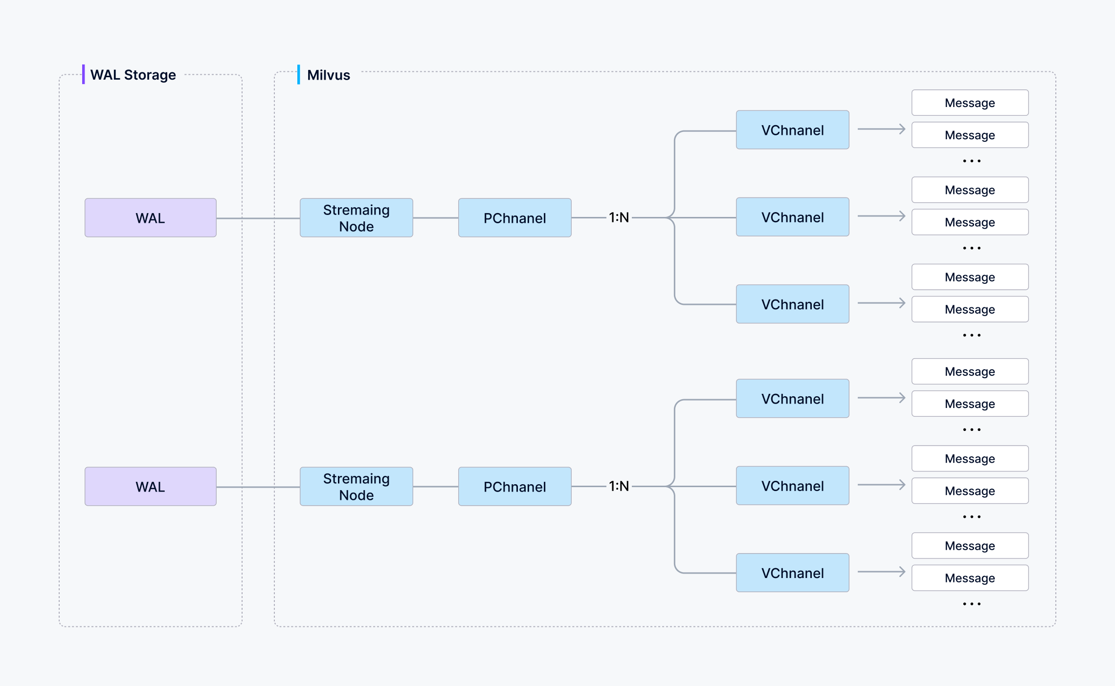
After data verification, the proxy will split the written message into various data package of shards according to the specified shard routing rules.
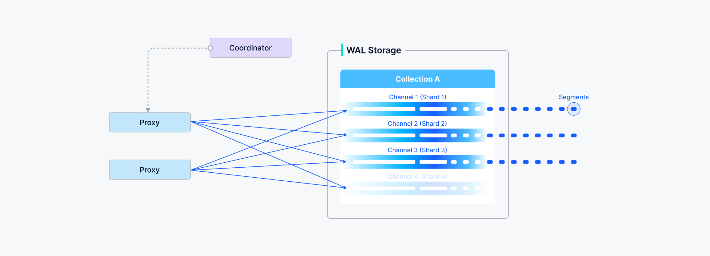
Then the written data of one shard (vchannel) is sent to the corresponding Streaming Node of pchannel.
The Streaming Node assigns a Timestamp Oracle (TSO) to each data packet to establish a total ordering of operations. It performs consistency checks on the payload before writing it into the underlying write-ahead log (WAL).
Meanwhile, the StreamingNode also asynchronously chops the committed WAL entries into discrete segments. There are two segment types:
- Growing segment: any data that has not been presisted into the object storage.
- Sealed segment: all data has been persisted into the object storage, the data of sealed segment is immutable.
The transition of a growing segment into a sealed segment is called a flush. The Streaming Node triggers a flush as soon as it has ingested and written all available WAL entries for that segment—i.e., when there are no more pending records in the underlying write-ahead log—at which point the segment is finalized and made read-optimized.
When the growing segment on a Streaming Node is flushed into a sealed segment—or when a Data Node completes a compaction—the Coordinator initiates a handoff operation to convert that growing data into historical data.
Index building
Index building is performed by data node. To avoid frequent index building for data updates, a collection in Milvus is divided further into segments, each with its own index.

Milvus supports building index for each vector field, scalar field and primary field. Both the input and output of index building engage with object storage: The data node loads the log snapshots to index from a segment (which is in object storage) to memory, deserializes the corresponding data and metadata to build index, serializes the index when index building completes, and writes it back to object storage.
Index building mainly involves vector and matrix operations and hence is computation- and memory-intensive. Vectors cannot be efficiently indexed with traditional tree-based indexes due to their high-dimensional nature, but can be indexed with techniques that are more mature in this subject, such as cluster- or graph-based indexes. Regardless its type, building index involves massive iterative calculations for large-scale vectors, such as Kmeans or graph traverse.
Unlike indexing for scalar data, building vector index has to take full advantage of SIMD (single instruction, multiple data) acceleration. Milvus has innate support for SIMD instruction sets, e.g., SSE, AVX2, and AVX512. Given the “hiccup” and resource-intensive nature of vector index building, elasticity becomes crucially important to Milvus in economical terms. Future Milvus releases will further explorations in heterogeneous computing and serverless computation to bring down the related costs.
Besides, Milvus also supports scalar filtering and primary field query. It has inbuilt indexes to improve query efficiency, e.g., Bloom filter indexes, hash indexes, tree-based indexes, and inverted indexes, and plans to introduce more external indexes, e.g., bitmap indexes and rough indexes.
Data query
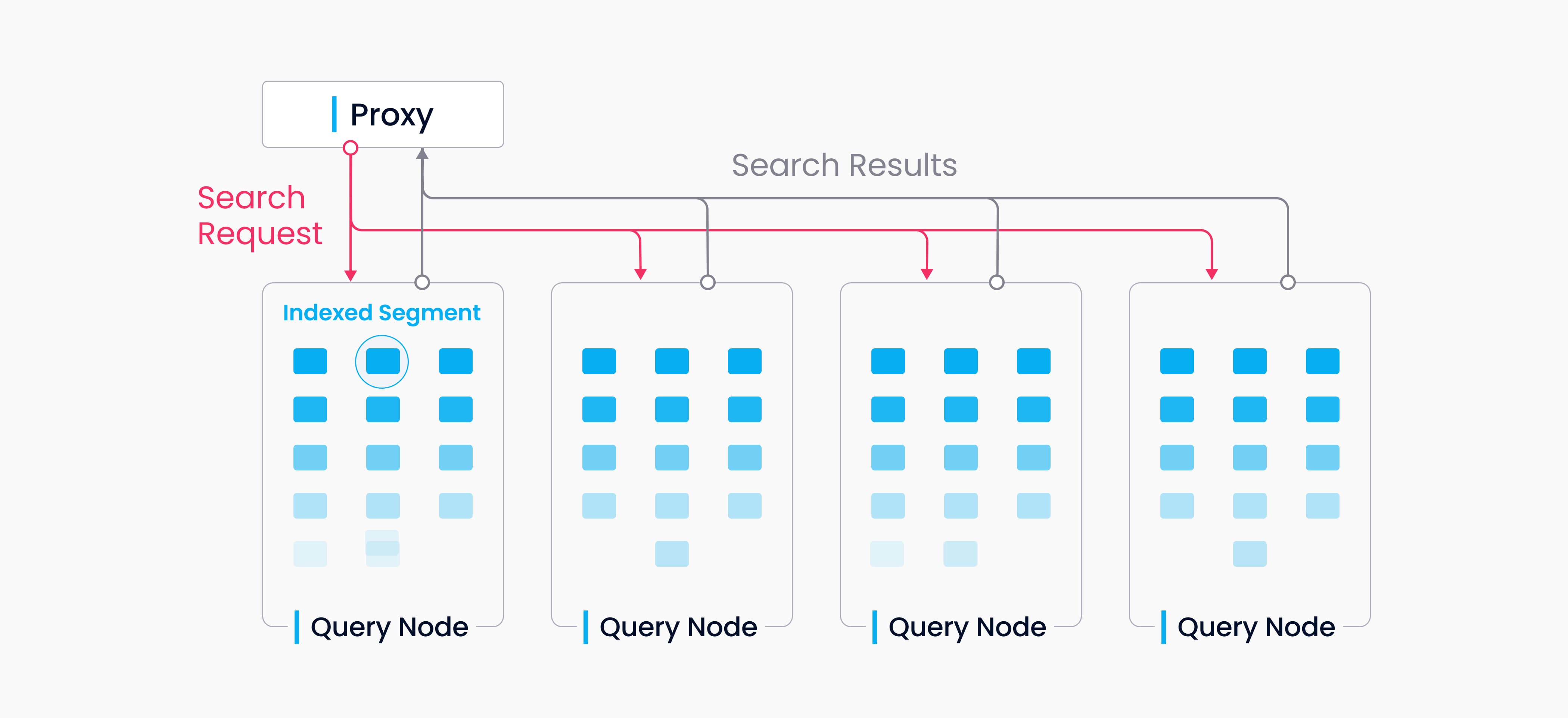
A collection in Milvus is split into multiple segments; the Streaming Node loads growing segments and maintains real-time data, while the Query Nodes load sealed segments.
When a query/search request arrives, the proxy broadcasts the request to all Streaming Nodes responsible for the related shards for concurrent search.
Each Streaming Node generates a query plan, searches its local growing data, and simultaneously contacts remote Query Nodes to retrieve historical results, then aggregates these into a single shard result.
Finally, the proxy collects all shard results, merges them into the final outcome, and returns it to the client.
Knowhere
Knowhere is the core vector execution engine of Milvus, which incorporates several vector similarity search libraries including Faiss, Hnswlib and Annoy. Knowhere is also designed to support heterogeneous computing. It controls on which hardware (CPU or GPU) to execute index building and search requests. This is how Knowhere gets its name - knowing where to execute the operations. More types of hardware including DPU and TPU will be supported in future releases.
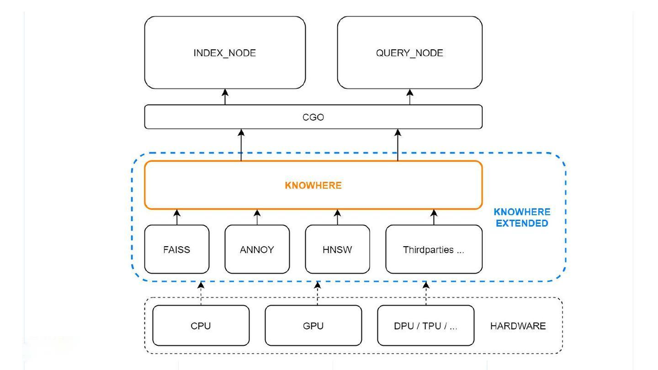
The bottom-most layer is the system hardware. Above this sit the third-party index libraries. At the top layer, Knowhere interacts with the index node and query node via CGO, which allows Go packages to call C code.
Bitset
In Milvus, bitsets are arrays of bit numbers 0 and 1 that can be used to represent certain data compactly and efficiently as opposed to in ints, floats, or chars. A bit number is 0 by default and is only set to 1 if it meets certain requirements.
Bitset is a simple yet powerful mechanism that helps Milvus perform attribute filtering, data deletion, and query with Time Travel.
Timestamp
When conducting a data manipulation language (DML) operation, including data insertion and deletion, Milvus assigns timestamps to the entities involved in the operation. Therefore, all entities in Milvus has a timestamp attribute. And the batches of entities in the same DML operation share the same timestamp value.
Guarantee_timestamp
Guarantee_timestamp is a type of timestamp used to ensure that all data updates by DML operations before the Guarantee_timestamp are visible when a vector similarity search or query is conducted.
If the Guarantee_timestamp is not configured, Milvus automatically takes the point in time when the search request is made. Therefore, the search is conducted on a data view with all data updates by DML operations before the search.
To save you the trouble of understanding the TSO inside Milvus, as a user, you do not have to directly configure the Guarantee_timestamp parameter. You only need to choose the consistency level, and Milvus automatically handles the Guarantee_timestamp parameter for you. Each consistency level corresponds to a certain Guarantee_timestamp value.

Service_timestamp
Service_timestamp is a type of timestamp automatically generated and managed by query nodes in Milvus. It is used to indicate which DML operations are executed by query nodes.
The data managed by query nodes can be categorized into two types:
- Historical data (or also called batch data)
- Incremental data (or also called streaming data).
In Milvus, you need to load the data before conducting a search or query. Therefore, batch data in a collection are loaded by query node before a search or query request is made. However, streaming data are inserted into or deleted from Milvus on the fly, which requires the query node to keep a timeline of the DML operations and the search or query requests. As a result, query nodes use Service_timestamp to keep such a timeline. Service_timestamp can be seen as the time point when certain data is visible as query nodes can ensure that all DML operations before Service_timestamp are completed.
When there is an incoming search or query request, a query node compares the values of Service_timestamp and Guarantee_timestamp.
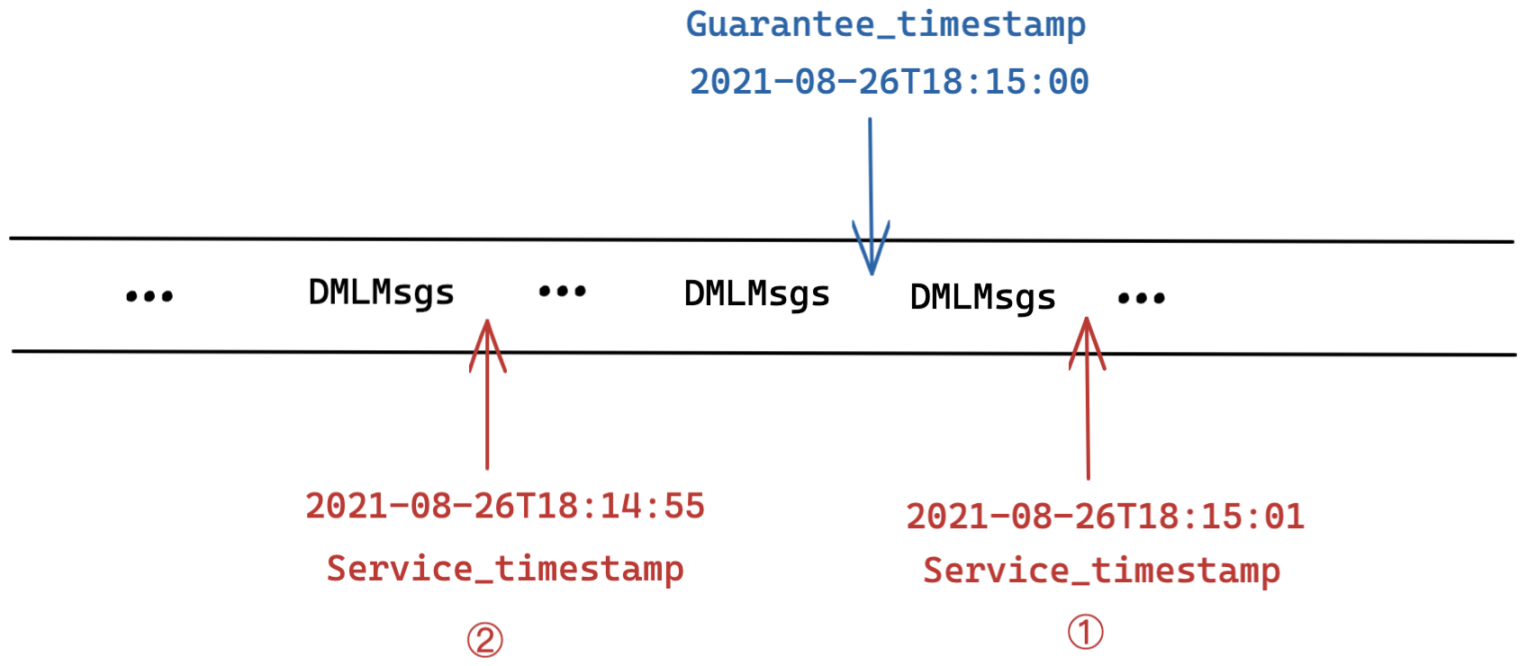
Scenario 1: Service_timestamp >= Guarantee_timestamp
As shown in the figure 1, the value of Guarantee_timestamp is set as 2021-08-26T18:15:00. When the value of Service_timestamp is grown to 2021-08-26T18:15:01, this means that all DML operations before this point in time are executed and completed by the query node, including those DML operations before the time indicated by Guarantee_timestamp. As a result, the search or query request can be executed immediately.
Scenario 2: Service_timestamp < Guarantee_timestamp
As shown in the figure 2, the value of Guarantee_timestamp is set as 2021-08-26T18:15:00, and the current value of Service_timestamp is only 2021-08-26T18:14:55. This means that only DML operations before 2021-08-26T18:14:55 are executed and completed, leaving part of the DML operations after this time point but before the Guarantee_timestamp unfinished. If the search or query is executed at this point, some of the data required are invisible and unavailable yet, seriously affecting the accuracy of the search or query results. Therefore, the query node needs to put off the search or query request until the DML operations before guarantee_timestamp are completed (i.e. when Service_timestamp >= Guarantee_timestamp).
Graceful_time
Technically speaking, Graceful_time is not a timestamp, but rather a time period (e.g. 100ms). However, Graceful_time is worth mentioning because it is strongly related to Guarantee_timestamp and Service_timestamp. Graceful_time is a configurable parameter in the Milvus configuration file. It is used to indicate the period of time that can be tolerated before certain data become visible. In short, uncompleted DML operations during Graceful_time can be tolerated.
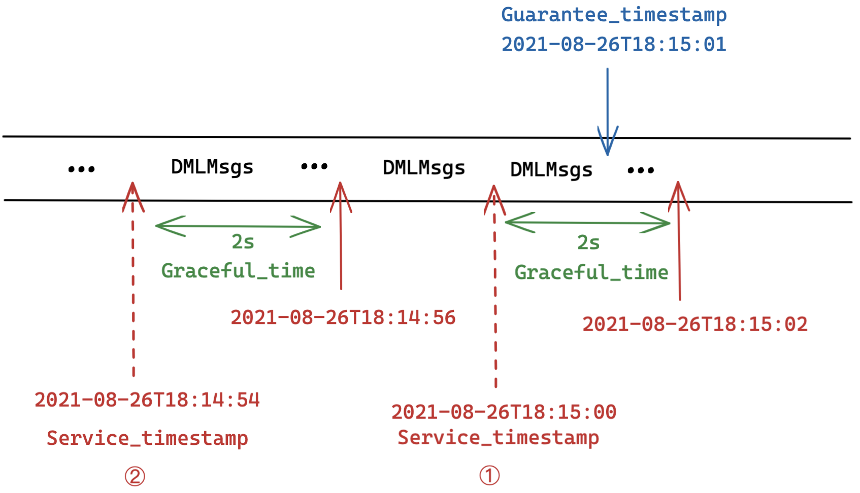
Scenario 1: Service_timestamp + Graceful_time >= Guarantee_timestamp
The value of Guarantee_timestamp is set as 2021-08-26T18:15:01, and Graceful_time as 2s. The value of Service_timestamp is grown to 2021-08-26T18:15:00. Though the value of Service_timestamp is still smaller than that of Guarantee_timestamp and not all DML operations before 2021-08-26T18:15:01 are completed, a period of 2 seconds of data invisibility is tolerated as indicated by the value of Graceful_time. Therefore, the incoming search or query request can be executed immediately.
Scenario 2: Service_timestamp + Graceful_time < Guarantee_timestamp
The value of Guarantee_timestamp is set as 2021-08-26T18:15:01, and Graceful_time as 2s. The current value of Service_timestamp is only 2021-08-26T18:14:54. This means that the expected DML operations are not completed yet and even given the 2 second of graceful time, data invisibility is still intolerable. Therefore, the query node needs to put off the search or query request until certain DML requests are completed (i.e. when Service_timestamp + Graceful_time >= Guarantee_timestamp).
Metrics
Similarity metrics are used to measure similarities among vectors. Choosing an appropriate distance metric helps improve classification and clustering performance significantly.
Currently, Milvus supports these types of similarity Metrics: Euclidean distance (L2), Inner Product (IP), Cosine Similarity (COSINE), JACCARD, HAMMING, and BM25 (specifically designed for full text search on sparse vectors).
| Field Type | Dimension Range | Supported Metric Types | Default Metric Type |
|---|---|---|---|
FLOAT_VECTOR | 2-32,768 | COSINE, L2, IP | COSINE |
FLOAT16_VECTOR | 2-32,768 | COSINE, L2, IP | COSINE |
BFLOAT16_VECTOR | 2-32,768 | COSINE, L2, IP | COSINE |
INT8_VECTOR | 2-32,768 | COSINE, L2, IP | COSINE |
SPARSE\_FLOAT\_VECTOR | No need to specify the dimension. | IP, BM25 (used only for full text search) | IP |
BINARY_VECTOR | 8-32,768*8 | HAMMING, JACCARD, MHJACCARD | HAMMING |
Index
HNSW(Hierarchical Navigable Small World)和IVF-Flat(Inverted File with Flat Index)是两种广泛应用于向量数据库的高效近似最近邻(ANN)搜索算法,它们在处理大规模高维向量数据时各有优劣。以下从核心原理、性能对比及适用场景三方面解析:
一、核心原理与技术特点
1. HNSW:分层导航小世界图
- 核心思想
结合跳表(Skip List) 和 可导航小世界图(NSW),构建多层图结构实现高效搜索:
- 分层设计:底层(Layer 0)包含所有节点,层级越高节点越稀疏,形成“高速公路式”快速路径。
- 贪心路由:从顶层入口点开始,每层选择距离查询向量最近的邻居节点,逐层向下精细化搜索。
- 动态更新:新数据插入时随机分配层级,仅需局部调整连接边(参数
M控制每层邻居数)。
- 关键参数
M:每层邻居数,影响索引精度和内存占用(值越大精度越高,内存消耗越大)。efConstruction:构建索引时的候选队列长度,决定索引质量。efSearch:搜索时的候选队列长度,直接影响召回率与延迟。
2. IVF-Flat:倒排文件+暴力搜索
- 核心思想
通过聚类预划分空间,缩小搜索范围:
- 空间分区:用k-means将向量空间划分为
nlist个聚类(簇),每个簇存储其质心和成员向量。 - 倒排索引:建立质心→向量的映射表,搜索时仅计算查询向量与最近质心对应簇内所有向量的距离(“Flat”即指无压缩的暴力计算)。
- 边界优化:通过参数
probes控制搜索的簇数量(如probes=5表示搜索最近的5个簇),平衡速度与召回率。
- 空间分区:用k-means将向量空间划分为
- 关键参数
nlist:聚类数量,影响索引构建速度和搜索精度(值越大精度越高,但构建更慢)。probes:搜索的簇数量,值越大召回率越高,但延迟增加。
二、性能对比与适用场景
| 维度 | HNSW | IVF-Flat |
|---|---|---|
| 搜索速度 | ⚡️ 极快(对数复杂度 O(log N)) | ⚡ 快(仅搜索部分簇,但仍需遍历簇内所有向量) |
| 索引构建时间 | ⏳ 慢(需构建多层图) | ⏱️ 极快(仅需一次聚类) |
| 内存占用 | 🧠 高(存储多层图结构) | 💾 低(仅存储原始向量+质心映射) |
| 精度/召回率 | ✅ 高(尤其适合高维数据) | ⚖️ 中等(依赖probes参数) |
| 动态更新 | ✅ 支持实时插入/删除 | ❌ 需定期重建索引(频繁更新导致精度下降) |
| 适用数据规模 | 百万~十亿级向量 | 千~百万级向量 |
三、典型应用场景选择建议
- 优先选择 HNSW 的场景
- 高精度需求:如RAG系统的知识库检索、推荐系统的实时召回。
- 动态数据环境:需频繁增删向量(如用户画像实时更新)。
- 资源充足:可接受较高内存消耗和较慢的索引构建(如云服务器部署)。
- 优先选择 IVF-Flat 的场景
- 中小规模数据(<100万向量)且需低成本部署。
- 静态数据集:数据更新频率低(如历史档案检索)。
- 速度与内存敏感:边缘设备或内存受限环境。
四、实际案例说明
- HNSW 在 RAG 系统中的应用 Weaviate 使用 HNSW 作为默认索引,在千万级文档库中实现毫秒级语义搜索。用户提问向量化后,通过分层导航快速定位相关文本块,显著提升大模型回答质量。
- IVF-Flat 在图像检索中的实践
百万级商品图片库使用 IVF-Flat 索引,以
nlist=1000划分聚类。用户上传图片后,仅需扫描最近3个簇(probes=3),即可在50ms内返回相似商品,兼顾效率与成本。
五、进阶调优策略
- HNSW 参数优化:
大数据集建议
M=16~32,efConstruction=200~400,搜索时efSearch=50~100平衡速度与召回。 - IVF-Flat 参数优化:
若召回不足,逐步增加
probes(不超过nlist的10%)。 - 混合索引方案(如 Milvus):
先用 IVF 粗筛(
probes=5)减少候选集,再用 HNSW 精搜,综合二者优势。
💎 总结:HNSW 以内存换速度与精度,适合大规模动态数据;IVF-Flat 以精度换内存与构建速度,适合中小规模静态数据。实际选型需结合数据规模、更新频率、硬件资源综合决策。
FastJson
Milvus 依赖 FastJSON 但不会自动导入该依赖,这主要源于其依赖管理策略、版本兼容性设计及 Java 生态的通用规范。以下是具体原因及技术解析:
🔧 1. 依赖作用域(Scope)设计
显式依赖原则 Milvus SDK 或相关模块(如
spring-ai-milvus-store)在设计时通常将 FastJSON 标记为 **provided作用域(Maven)或 compileOnly**(Gradle)。这意味着:- FastJSON 是运行时必需的,但 SDK 不强制绑定其版本。
- 用户需根据自身项目环境显式引入 FastJSON,以避免版本冲突。
<!-- Maven 示例:Milvus SDK 可能隐含的依赖声明 -->
<dependency>
    <groupId>com.alibaba</groupId>
    <artifactId>fastjson</artifactId>
    <version>[用户自定]</version>
    <scope>provided</scope> <!-- 不自动传递依赖 -->
</dependency>
避免依赖地狱 FastJSON 的版本更新频繁且存在安全风险(如反序列化漏洞)。若 Milvus 强制绑定特定版本,可能导致:
- 用户项目中的其他库因版本冲突而失效。
- 安全漏洞无法通过升级 FastJSON 独立修复。
⚙️ 2. 模块化与轻量化考量
- 减少 SDK 体积 Milvus SDK 核心功能聚焦于向量操作和数据库连接,若打包 FastJSON 会增大分发体积。用户可选择更小的替代库(如 Jackson)或按需引入 FastJSON。
- 灵活适配 JSON 库 部分企业已标准化 JSON 库(如 Spring Boot 默认使用 Jackson)。Milvus 不强制依赖 FastJSON 允许用户无缝集成现有技术栈。
🛡️ 3. 安全与版本兼容性
规避高危版本
FastJSON 旧版本(如 ≤1.2.68)存在严重漏洞(如 CVE-2017-18349)。Milvus 通过
不自动引入
的方式:
促使用户主动选择安全版本(如 ≥2.0.47)。
避免因 SDK 内置旧版本导致安全风险。
版本兼容性挑战 Milvus 的 JSON 序列化逻辑可能依赖 FastJSON 特定 API(如
JSONWriter.Feature)。若自动绑定版本,用户升级 SDK 时可能因 API 变更而崩溃。
🔄 4. 构建工具的限制
Maven/Gradle 的依赖传递机制
即使 Milvus SDK 声明了 FastJSON 依赖,若其作用域为
provided
或
compileOnly
,构建工具
不会将其打包到最终应用
中。用户需在项目中显式添加:
// Gradle 示例
implementation 'com.alibaba:fastjson:2.0.47'
- 本地仓库缓存问题
若用户本地 Maven 仓库(
~/.m2/repository)缺失 FastJSON,即使 SDK 声明依赖,构建时仍会报错NoClassDefFoundError。
💎 总结:Milvus 的设计逻辑与用户应对
Milvus 不自动导入 FastJSON 是权衡灵活性、安全性和兼容性的结果。开发者需:
- 显式添加依赖:在
pom.xml或build.gradle中引入 FastJSON。 - 锁定安全版本:优先使用 ≥2.0.47 的 FastJSON2。
- 验证依赖树:通过
mvn dependency:tree检查版本冲突。 - 替代方案:若需换用 Jackson,需重写 Milvus 的序列化适配层(需修改源码)。
graph TD
    A[Milvus 依赖 FastJSON] --> B{是否自动导入?}
    B -->|否| C[原因1:作用域设为 provided]
    B -->|否| D[原因2:避免版本冲突]
    B -->|否| E[原因3:安全风险规避]
    C --> F[用户需显式添加依赖]
    D --> F
    E --> F
    F --> G[项目构建成功]
标量默认索引
在 Milvus 中,标量字段(非向量字段)的默认索引策略是自动索引(Auto Index),系统会根据标量字段的数据类型自动选择最优的索引类型,无需用户手动指定。这一策略旨在简化配置并适配常见查询场景。以下是具体规则和细节:
📌 一、默认索引策略:自动索引(Auto Index)
触发条件 当创建索引时不指定
index_type参数或将其留空,Milvus 会启用自动索引机制。数据类型与索引类型的映射 Milvus 根据字段数据类型自动选择索引算法,对应关系如下:
标量字段数据类型 自动选择的索引类型 适用场景 VARCHAR(字符串)倒排索引(Inverted) 等值查询、前缀匹配、范围查询 INT8/16/32/64(整数类型)倒排索引(Inverted) 精确匹配、范围查询(如 id > 100)FLOAT/DOUBLE(浮点数)倒排索引(Inverted) 范围查询(如 price BETWEEN 10.0 AND 50.0)BOOL(布尔值)倒排索引(Inverted) 布尔条件过滤(如 status = True)ARRAY(数组)倒排索引(Inverted) 数组元素的等值或包含查询 💡 说明:倒排索引通过构建“术语字典+倒排列表”加速查询,尤其适合点查询和范围过滤,性能比暴力搜索提升显著(实验显示点查询快30倍)。
⚠️ 二、注意事项
- 不支持的数据类型
JSON类型无法创建标量索引,需通过其他方式处理。 - 每个字段仅支持一个索引
若需更换索引类型(如改用
BITMAP或TRIE),需先删除现有索引。 - 自动索引的局限性
- 虽简化配置,但特定场景需手动优化:
- 低基数(Cardinality < 500)字段 → 改用
BITMAP索引提升等值查询效率。 - 字符串前缀搜索 → 手动指定
TRIE索引更高效。
- 低基数(Cardinality < 500)字段 → 改用
- 浮点字段不支持
BITMAP索引(因二进制不兼容)。
- 虽简化配置,但特定场景需手动优化:
💎 三、总结
- 默认策略:
Auto Index→ 按数据类型自动选择 倒排索引。 - 核心优势:降低配置复杂度,适配多数场景(尤其文本、数值的过滤查询)。
- 手动优化场景:低基数字段、字符串前缀匹配、超高基数(>500)字段需自定义索引类型。
建议通过 list_indexes() 验证索引创建结果,例如:
# 查看集合全部索引
indexes = client.list_indexes(collection_name="your_collection")
print(indexes)  # 输出示例:['default_index']
标量索引
Milvus 为标量字段(如数值、字符串、布尔值等非向量数据)提供了多种索引类型,用于加速标量过滤和查询操作。以下是其支持的 5 种标量索引方式及其核心特点与适用场景:
🔍 1. 自动索引(Auto Index)
特点: Milvus 根据字段数据类型自动选择最优索引类型,无需用户指定,简化配置流程。
适用场景
:
通用型字段(如数值、字符串、布尔值)。
快速原型验证或对索引类型无特殊要求的场景。
数据类型支持:
INT8/16/32/64、FLOAT/DOUBLE、BOOL、VARCHAR、ARRAY。
🔢 2. 倒排索引(Inverted Index)
特点: 通过“术语字典+倒排列表”结构,高效支持等值查询(
category == 1)和范围查询(price > 50.0)。
适用场景
:
高频过滤字段(如分类标签、用户评分)。
高基数(不同值数量多)或混合查询需求。
数据类型支持: 所有标量类型(除
JSON外),包括数值、字符串、布尔值和数组。
🧩 3. 位图索引(Bitmap)
特点: 为每个唯一值生成二进制位图,通过位运算(如
AND/OR)快速合并多条件查询。
适用场景
:
低基数字段(如性别、状态标志),基数建议 < 500。
多条件组合查询(如
status=True AND category="A")。
限制
:
- 不支持浮点类型(
FLOAT/DOUBLE)和JSON。 - 高基数字段会导致存储开销激增。
🔤 4. 前缀树索引(Trie)
特点: 基于树形结构优化字符串前缀匹配(如
name LIKE "apple%")。
适用场景
:
VARCHAR字段的前缀搜索或精确匹配。文本标签、产品名称等字符串类目过滤。
限制: 不支持数值范围查询(如
price > 100)。
📊 5. STL_SORT 索引
特点: 利用排序算法优化数值字段的范围查询和排序操作(如
ORDER BY timestamp)。
适用场景
:
数值字段的范围过滤(如时间戳、价格区间)。
需要排序结果的查询。
数据类型支持:
BOOL、INT8/16/32/64、FLOAT、DOUBLE。
⚙️ 索引选择与使用建议
| 索引类型 | 适用数据类型 | 典型查询场景 | 基数要求 |
|---|---|---|---|
| 自动索引(Auto) | 通用类型 | 快速部署,无特殊优化需求 | 任意 |
| 倒排索引(Inverted) | 所有标量(除 JSON) | 等值/范围混合查询 | 高/低基数均可 |
| 位图索引(Bitmap) | 整数、布尔、短字符串 | 多条件组合查询 | 低基数(<500) |
| 前缀树(Trie) | VARCHAR | 前缀匹配(LIKE "prefix%") | 中低基数 |
| STL_SORT | 数值类型 | 范围查询/排序 | 任意 |
特殊限制
:
JSON类型仅支持倒排索引。位图索引不支持浮点数。
操作建议
:
- 使用
list_indexes()验证索引是否创建成功。 - 每个字段仅支持一个索引,更换类型需先删除旧索引。
💎 总结
Milvus 的标量索引策略覆盖了从自动化配置(Auto Index)到针对特定场景(如字符串前缀、低基数枚举、数值排序)的专项优化。倒排索引是默认且最通用的选择,而位图索引在低基数多条件查询中性能最优。实际应用中需结合字段数据类型、基数分布及查询模式综合选择,必要时可通过 list_indexes() 接口验证索引状态。
索引物理结构
Milvus 的索引底层物理结构因索引类型和目标数据类型(向量或标量)而异,其设计核心在于高效支持相似性搜索和标量过滤。以下是主要索引类型的底层物理结构详解:
⚙️ 一、向量索引的物理结构
向量索引主要用于加速高维向量的近似最近邻搜索(ANN),其物理结构取决于具体算法:
HNSW(分层导航小世界图)
 结构

 :多层图结构(Hierarchical Graph)。

 - 底层(第0层)包含全量数据点,连接密集;
 - 上层(第1层及以上)逐步稀疏化,节点间连接距离递增。
 关键参数

 :

 - `M`:每层节点的最大连接数(影响图密度和精度);
 - `efConstruction`:构建时的搜索范围(影响索引质量)。
- 适用场景:高精度搜索,内存资源充足(如百万级数据集)。
IVF 系列(倒排文件索引)
 结构

 :基于聚类的倒排列表(Inverted Lists)。

 - 数据被划分为 `nlist` 个聚类中心(质心);
 - 每个聚类对应一个倒排列表,存储属于该簇的向量ID及原始向量或量化后的值。
 子类型差异

 :

 - **IVF_FLAT**:存储原始向量,无压缩;
 - **IVF_SQ8**:标量量化(Scalar Quantization),将浮点数压缩为8位整数;
 - **IVF_PQ**:乘积量化(Product Quantization),向量分段压缩。
- 查询流程:先定位最近质心,再扫描对应倒排列表。
FLAT(暴力搜索)
- 结构:原始向量连续数组(Flat Array)。
- 无额外数据结构,直接计算查询向量与全量数据的距离,适用于极小数据集(≤1万条)。
稀疏向量索引(SPARSE_INVERTED_INDEX)
 结构

 :维度级倒排列表(Dimension-wise Inverted Lists)。

 - 每个维度维护一个列表,记录在该维度非零的向量ID及值。
- 优化:通过
drop_ratio参数忽略低权重值,平衡精度与速度。
🔢 二、标量索引的物理结构
标量索引用于加速结构化字段(如整数、字符串)的过滤:
倒排索引(INVERTED)
 结构

 :词项字典(Term Dictionary)+ 倒排列表(Posting Lists)。

 - 字典存储唯一值(如 `category="A"`);
 - 倒排列表存储包含该值的文档ID集合。
- 适用:等值查询(
age=30)、范围查询(price>100)。
位图索引(BITMAP)
 结构

 :位向量数组(Bit Vector Arrays)。

 - 每个唯一值对应一个位向量,标记包含该值的行(如 `[1,0,1]` 表示第0、2行满足条件)。
- 优势:支持多条件位运算(AND/OR),适合低基数字段(如性别)。
前缀树索引(TRIE)
 结构

 :多叉树(Trie Tree)。

 - 节点存储字符,路径表示字符串前缀(如 "app" → "apple")。
- 适用:字符串前缀匹配(
LIKE "abc%")。
STL_SORT 索引
 结构

 :排序数组(Sorted Array)。

 - 数据按字段值排序存储,支持二分查找加速范围查询。
- 适用:数值字段的范围过滤或排序(
ORDER BY timestamp)。
🧩 三、索引的存储与执行流程
- 持久化存储:
- 索引文件(如 IVF 的聚类数据、HNSW 的图结构)以二进制形式存入对象存储(如 MinIO/S3)。
- 元数据(索引类型、参数)保存在 etcd 中。
- 查询加载:
- 查询时,Query Node 将索引文件从对象存储加载到内存,并根据索引类型执行搜索:
- HNSW:图遍历;
- IVF:定位聚类→扫描倒排列表;
- 倒排索引:检索倒排列表。
- 查询时,Query Node 将索引文件从对象存储加载到内存,并根据索引类型执行搜索:
💎 四、总结:索引结构与适用场景
| 索引类型 | 底层物理结构 | 典型应用场景 | 关键设计目标 |
|---|---|---|---|
| HNSW | 多层图结构 | 高精度向量搜索 | 平衡召回率与查询延迟 |
| IVF_FLAT/PQ/SQ8 | 聚类中心+倒排列表 | 大规模向量数据集 | 压缩存储,降低内存占用 |
| 倒排索引 (INVERTED) | 词项字典+倒排列表 | 标量等值/范围过滤 | 加速多值匹配 |
| 位图索引 (BITMAP) | 位向量数组 | 低基数字段的多条件过滤 | 位运算高效合并 |
| TRIE | 前缀树 | 字符串前缀匹配 | 减少字符扫描次数 |
设计共性:
- 冷热分离:索引文件存储在对象存储(冷数据),查询时加载到内存(热数据)。
- 异步构建:索引由 Index Node 异步生成,避免阻塞数据写入。
- 参数化调优:通过
nlist、M、ef等参数平衡精度、速度与资源。
如需进一步优化索引性能,可结合字段基数、查询模式调整参数(如低基数用 BITMAP,高精度用 HNSW)。
JSON 索引
在 Milvus 中,JSON 类型字段的索引是通过 路径索引(Path Indexing) 实现的,允许针对 JSON 结构内的特定字段(如嵌套键或数组元素)创建索引以加速查询。以下是具体机制和操作指南:
⚙️ JSON 字段索引的核心机制
- 索引类型
- 仅支持 倒排索引(INVERTED)。
- 通过指定 JSON 路径(
json_path)和数据类型(json_cast_type),提取目标值并构建索引。
- 路径索引原理
- 索引针对 JSON 内部的特定路径(如
metadata["product_info"]["category"]),而非整个 JSON 对象。 - 示例:为
metadata.price创建数值索引后,查询metadata["price"] > 100可直接命中索引。
- 索引针对 JSON 内部的特定路径(如
🔧 如何为 JSON 的特定字段创建索引?
通过以下步骤实现针对单一字段的索引:
定义索引参数
index_params = client.prepare_index_params() index_params.add_index( field_name="metadata", # JSON 字段名 index_type="INVERTED", # 仅支持倒排索引 index_name="price_index", # 自定义索引名 params={ "json_path": "metadata[\"price\"]", # 指定目标字段路径 "json_cast_type": "double" # 转换数据类型 } )参数说明:
json_path:需索引的 JSON 路径(支持嵌套键和数组,如tags[0])。json_cast_type:目标数据类型(varchar、double或bool)。
创建索引
client.create_index(collection_name="my_collection", index_params=index_params)
⚠️ 关键注意事项
数据类型匹配
查询条件必须与
json_cast_type一致,否则索引失效:
- 若索引类型为
double,则过滤条件需为数值(如metadata["price"] > 100)。 - 若为
varchar,则需字符串条件(如metadata["category"] == "electronics")。
- 若索引类型为
数据一致性要求
- 类型不一致:若某行数据的路径值类型与
json_cast_type不符(如字符串存入数值索引),该行将被跳过索引。 - 路径缺失:路径不存在的数据行不会被索引,但不会报错。
- 类型不一致:若某行数据的路径值类型与
数值精度限制
- 数值类型(如
double)索引存在精度限制(超过 2^53 的整数可能丢失精度),需避免大整数场景。
- 数值类型(如
数组索引限制
- 当前不支持数组整体索引(如
tags数组),仅支持索引数组中的标量元素(如tags[0])。
- 当前不支持数组整体索引(如
🚀 高级技巧:动态字段的索引
若启用动态字段(enable_dynamic_fields=True),未定义的字段会存入 $meta JSON 中,可通过相同方式索引:
index_params.add_index(
    field_name="color",             # 动态字段名(如 color)
    index_type="INVERTED",
    params={
        "json_path": "color",       # 直接指定键名
        "json_cast_type": "varchar"
    }
)
动态字段的查询语法与普通字段相同(如 color == "red")。
💎 总结与建议
- 索引场景:对高频查询的 JSON 路径(如分类、价格)单独建索引,避免全表扫描。
- 路径选择:优先索引低基数、高频过滤的字段(如
category而非description)。 - 数据类型:根据实际查询需求选择
json_cast_type(字符串选varchar,数值选double)。 - 性能平衡:每个新增索引会增加存储开销,建议按需创建。
通过精准的路径索引,JSON 字段的过滤性能可提升数十倍。例如,为
metadata["price"]建索引后,范围查询速度接近常量时间复杂度。